Logistic Regression
Logistic regression models the log-odds of an event as a linear combination of variables. For a single observation, the model is:
\[ \log\left(\frac{p_i}{1 - p_i}\right) = x_i^\top \beta \]
Here, \(x_i\) is a vector of input features for the \(i^{th}\) observation, and \(p_i\) is the predicted probability that the outcome equals 1 for that observation. Across all \(n\) observations, we can write this compactly as:
\[ \log\left(\frac{p}{1 - p}\right) = X\beta \]
where \(X\) is an \(n \times (\nu + 1)\) matrix of inputs, \(\beta\) is a \((\nu + 1) \times 1\) coefficient vector, and \(p\) is an \(n \times 1\) vector of predicted probabilities.
Solving for \(p\), we get:
\[ p = \frac{e^{X\beta}}{1 + e^{X\beta}} \]
This sigmoid function maps the linear predictor to a probability between 0 and 1. To classify observations, we apply a threshold—commonly 0.5—on \(p\). In our Human-vs-Bot project, we define bots as the positive class (\( \text{isBot} = 1 \)), so a probability above a threshold of 0.5 indicates a likely bot.
Threshold determination
Deciding where to place a cut-point is not always straightforward. A cut-point determines which cases get classified as positive—that is, which logit score (and associated probability) best separates the two classes. In our model, this means deciding what score most effectively distinguishes a human from a bot. How can we maximize predictive accuracy?
Often, it's important to evaluate several candidate thresholds and assess how the model performs at each. This involves examining classification metrics such as sensitivity (true positive rate), specificity (true negative rate), and predictive values. All of these metrics are defined relative to a particular threshold.
To assess overall model discrimination independent of any specific cut-point, we use the area under the receiver operating characteristic (ROC) curve, or AUC. AUC represents the probability that a randomly selected positive case (e.g., bot) will be assigned a higher predicted probability than a randomly selected negative case (e.g., human).
Accuracy, often mistaken for predictive performance, summarizes the proportion of correctly classified cases—true positives and true negatives combined—divided by the total number of cases. However, it doesn’t indicate whether the model systematically misclassifies one group more than the other, and it can be especially misleading when one class is much smaller than the other.
Predictive performance requires a specific cut-point. The positive predictive value (PPV) is the proportion of predicted positives that are actual positives (i.e., predicted bots that actually are bots), while the negative predictive value (NPV) is the proportion of predicted negatives that are truly negative (i.e., predicted humans that actually are humans). These metrics depend both on the chosen threshold and the underlying class distribution. In machine learning contexts, PPV is often called precision, and sensitivity is referred to as recall.
A decision table is a practical tool for comparing potential cut-points. It lists a range of thresholds (e.g., 0.0, 0.1,..., 1.0 for probabilities—though logit scores may also be used) alongside key metrics such as True Positive Rate (TPR; sensitivity; recall), False Positive Rate (FPR), Positive Predictive Value (PPV; precision), and Negative Predictive Value (NPV).
For instance, a cut-point of 0.0 classifies all cases as bots, maximizing TPR but also FPR, which results in low PPV due to many false positives. A cut-point of 1.0 classifies no cases as bots, yielding both TPR and FPR of 0, and high NPV—but no positive predictions. Intermediate thresholds like 0.5 attempt to balance these metrics.
The optimal cut-point depends on project priorities—whether it’s more important to detect bots or to minimize false positives. For this project, we use a conventional threshold of 0.5: probabilities greater than 0.5 classify a case as a bot. This threshold will be used below to construct a confusion matrix and evaluate predictive performance.
To further explore classification beyond logistic regression—including models with more flexible decision boundaries and different learning biases—see the Machine Learning section.
Results
Model Selection
We fit two logistic models for our data: one using only the predictor, response rate (rate), and another using both, response rate and standard deviation of inter-response times (rate & sd_inter_response).
            Call:
            glm(formula = isBot ~ rate, family = "binomial", data = training_data)

            Coefficients:
                    Estimate Std. Error z value Pr(>|z|)
            (Intercept) 0.003402   0.098073   0.035    0.972
            rate        0.214539   0.202490   1.060    0.289

            (Dispersion parameter for binomial family taken to be 1)

            Null deviance: 775.87  on 559  degrees of freedom
            Residual deviance: 774.61  on 558  degrees of freedom
            AIC: 778.61

            Number of Fisher Scoring iterations: 4
            Call:
            glm(formula = isBot ~ rate + sd_inter_response, family = "binomial",
                data = training_data)

            Coefficients:
                   Estimate Std. Error z value Pr(>|z|)
            (Intercept)     18.8576     1.6917  11.147   <2e-16 ***
            rate            -7.9457     0.9557  -8.314   <2e-16 ***
            sd_inter_response  -1.6746     0.1563 -10.711   <2e-16 ***
            ---
            Signif. codes:  0 ‘***’ 0.001 ‘**’ 0.01 ‘*’ 0.05 ‘.’ 0.1 ‘ ’ 1

            (Dispersion parameter for binomial family taken to be 1)

            Null deviance: 775.87  on 559  degrees of freedom
            Residual deviance: 245.69  on 557  degrees of freedom
            AIC: 251.69

            Number of Fisher Scoring iterations: 7
In the first model, rate is not statistically significant (p = 0.289). However, when sd_inter_response is included as a second predictor, both rate and sd_inter_response become highly significant (p < 0.001). Additionally, the second model's AIC (251.69) is substantially lower than the first model's (778.61), indicating a much better fit. This suggests that the combination of response rate and variability in response timing provides stronger predictive power than response rate alone. Thus, our final model is:
\[ \log\left(\frac{p}{1 - p}\right) \approx -7.95\cdot\text{rate} - 1.67\cdot\text{sd_inter_response} \]
sd_inter_response).
This can be re-written in terms of probability as seen above:
\[p = \frac{e^{-7.95\cdot\text{rate} - 1.67\cdot\text{sd_inter_response}}}{1 + e^{-7.95\cdot\text{rate} - 1.67\cdot\text{sd_inter_response}}}\]
This is just one model built using one method among many possible options. Before using it to support forecasting or decision-making, we need to evaluate how well it generalizes to new data. This logistic model was trained on one portion of the data; we now assess its performance on an independent test set. While more advanced techniques—such as k-fold cross-validation—can be used during training to improve robustness, we do not cover those in this project.
ROC Curve
Using the description above, with an AUC of 0.94, we can say that 94% of the time, when we randomly select one bot and one human case, the model assigns a higher score to the bot. But what counts as a “good” AUC depends a lot on what you're modeling. Take recidivism: regular recidivism is difficult to predict, and violent recidivism is more difficult. So an AUC of 0.6 in that context might be acceptable, depending on what's at risk. But for something like human vs. bot response behavior, an AUC of 0.94 is—at the very least—pretty solid.
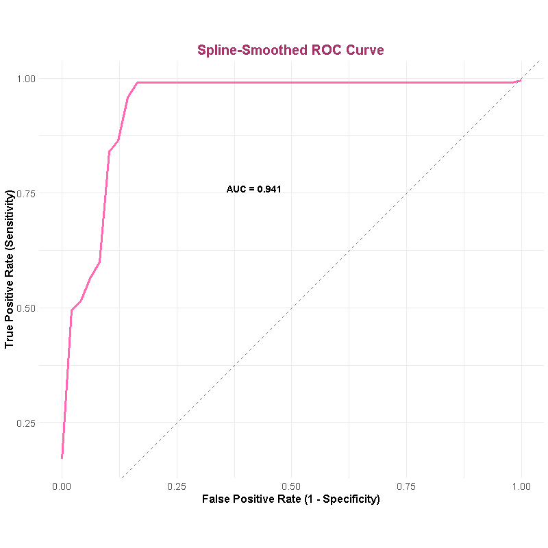
As mentioned earlier, AUC is a threshold-independent measure. It evaluates the model’s ability to distinguish between classes by plotting sensitivity (recall) against the false positive rate (1 - specificity) across all possible thresholds. While this provides a useful summary of discrimination, it doesn’t reflect how the model performs at any specific cut-point.
In practice, classification models are often used to make discrete predictions—such as labeling a case as "bot" or "human"—and this requires selecting a threshold. Once a cut-point is chosen, we can assess the model's predictive performance using metrics like precision, recall, and predictive values. These metrics are dependent on that chosen threshold and offer a more practical view of how the model behaves in real-world decision-making.
Decision Table
The decision table below displays all predictive and ROC-based values across a range of cut-points.
If we choose a probability of 0.5 (probability scores strictly above 0.5) as the cut-off for classification, then we can expect that 85% of the cases classified as bots are indeed bots — this is the positive predictive value (PPV), also referred to as precision. The negative predictive value (NPV) of 0.98 indicates that 98% of the cases predicted to be human are actually human. This implies a false negative rate of 2% among predicted humans — that is, 2% of those classified as human are actually bots.
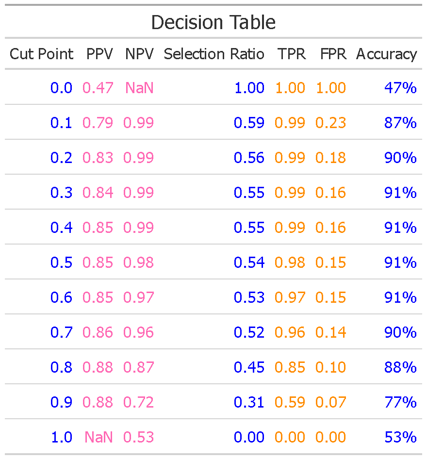
You may notice that the positive or negative predictive value (PPV or NPV) appears as NaN (Not a Number) at extreme cut-points of 0 and 1. This is not an error—it’s a mathematically valid result. For example, at a cut-point of 0 (i.e., classifying all cases as bots), no cases are predicted as human. The negative predictive value (NPV) is defined as the proportion of predicted negative (humans) that are actually negative. When we place all cases into the positive class (bot class), there are no cases left for asssessment: the NVP calculation considers the number of cases predicted as human. At a cutpoint of zero, no cases were predicted (classified) as human—they are are classified as bots—and we are essentially dividing my zero: resulting in an undefined value (NaN) The same logic applies at a cut-point of 1, where all cases are classified as human. In this case, PPV becomes undefined because there are no predicted positives (bots), leaving the denominator in the PPV formula equal to zero.
Once a cutpoint is selected, a confusion matrix can be constructed. A confusion matrix is a two by two table of the outcomes: predicted outcomes and actual outcomes. The outcomes are with respect to what our model was predicting, in this case, human or bot response behavior. In each cell of the 2x2 table is a count: the true positive and true negative are on one diagnol and false negatives and false positives on the other daignol.
| Actual: Human | Actual: Bot | |
|---|---|---|
| Predicted: Human | True Positive | False Negative |
| Predicted: Bot | False Positive | True Negative |
We constructed a confusion matrix in R using a cut-off of 0.5. That is, if we classify cases with model scores at or below 0.5 as human, and those above 0.5 as bots, the resulting confusion table appears as follows.
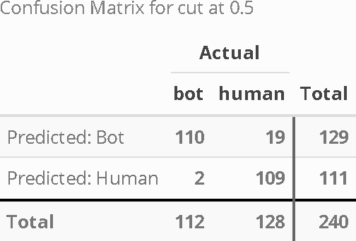
Accuracy is the total number of correct classifications (true positives + true negatives) divided by the total number of cases.
\[ Accuracy = \frac{tp + tn}{n} \]
\[ Accuracy = \frac{110 + 109}{240}\\ = 0.9125 \]
\[ PPV = \frac{tp + tn}{129} = 0.8527 \]
The negative predictive value, false positive, and false positive rates can also be calculated from the confusion trable.
Limitations
While logistic regression is interpretable and effective for linearly separable data, it has several limitations that are worth addressing:
- Linearity Assumption: Logistic regression assumes a linear relationship between the input variables and the log-odds of the response. This may not hold true if the data contains complex or nonlinear patterns, in which case more flexible models like tree-based methods might perform better.
- Multicollinearity: Strong correlation between predictors can destabilize coefficient estimates, making interpretation difficult and potentially reducing model performance. Diagnostic checks or dimensionality reduction techniques (e.g., PCA) may be needed in such cases.
- Overfitting: Including too many features, especially irrelevant ones, can lead to overfitting. Regularization methods like L1 (Lasso) and L2 (Ridge) penalize large coefficients to help prevent this. However, we did not include regularization in the current model. A future extension of this project could incorporate regularized logistic regression to assess whether prediction improves or model coefficients become more robust.
- Threshold Sensitivity: While the ROC and AUC provide threshold-independent measures of discrimination, real-world decision-making depends on choosing a cut-point. Model performance can vary substantially depending on the threshold selected, especially in imbalanced datasets.
- Simulated Data: The data used here are synthetic. While they were generated to reflect plausible response behaviors, real-world data may introduce noise, variability, and distributional characteristics that this model hasn’t accounted for. Applying this model to real data would require recalibration and validation.
- Scalability: Logistic regression scales well to larger datasets, but with high-dimensional features or extremely large data volumes, specialized tools (e.g., stochastic gradient descent implementations, Spark MLlib) may be needed to ensure efficient computation.
Despite these limitations, logistic regression remains a strong baseline and a valuable tool for understanding model behavior. Enhancing this model with regularization and evaluating on more complex or realistic datasets are natural next steps.
While this page focuses on logistic regression, alternative classifiers (e.g., SVMs, Random Forests) may handle nonlinear or higher-dimensional patterns better—especially in real-world data.